2D Scatter Density as a Visual Conditional Independence Test (v26)
This writeup describes the solution I developed for the ADIA Lab Causal Discovery Challenge as part of my BSc thesis at VNU-UET (2026). The solution achieves 81.14% balanced accuracy locally and 80.82% on the CrunchDAO public leaderboard, surpassing the original competition top-1 result of 76.70% by +4.12%. A second post covers the Conv2D / 2D scatter density extension (v26).
Disclaimer
I had prior knowledge of the competition through the ADIA Lab survey paper, which describes the data-generating process. I did not use this to generate synthetic training data — that would invalidate the scientific contribution.
My solution is built directly on top of the top-1 competition writeup as a baseline. I also drew EDA insights and the XY augmentation idea from the 3rd-place writeup. The novelty claims in this post are incremental improvements on that foundation — I’d rather be honest about that than oversell it.
This blog post is written by Claude with me as a proofreader and editor. The technical content is my work, but the writing style is a collaboration.
All source code is available in this repository. All experiment results are in this Google Sheet.
Problem Setup
Given $n = 1000$ observations of $p \in {3, \ldots, 10}$ variables, where a causal edge $X \to Y$ is always known to exist, classify every other variable $K$ into one of 8 causal roles:
| Role | Graph motif |
|---|---|
| Confounder | $X \leftarrow K \rightarrow Y$ |
| Mediator | $X \rightarrow K \rightarrow Y$ |
| Collider | $X \rightarrow K \leftarrow Y$ |
| Cause of X | $K \rightarrow X$, no edge to $Y$ |
| Cause of Y | $K \rightarrow Y$, no edge to $X$ |
| Consequence of X | $X \rightarrow K$, no edge to $Y$ |
| Consequence of Y | $Y \rightarrow K$, no edge to $X$ |
| Independent | No edge to $X$ or $Y$ |
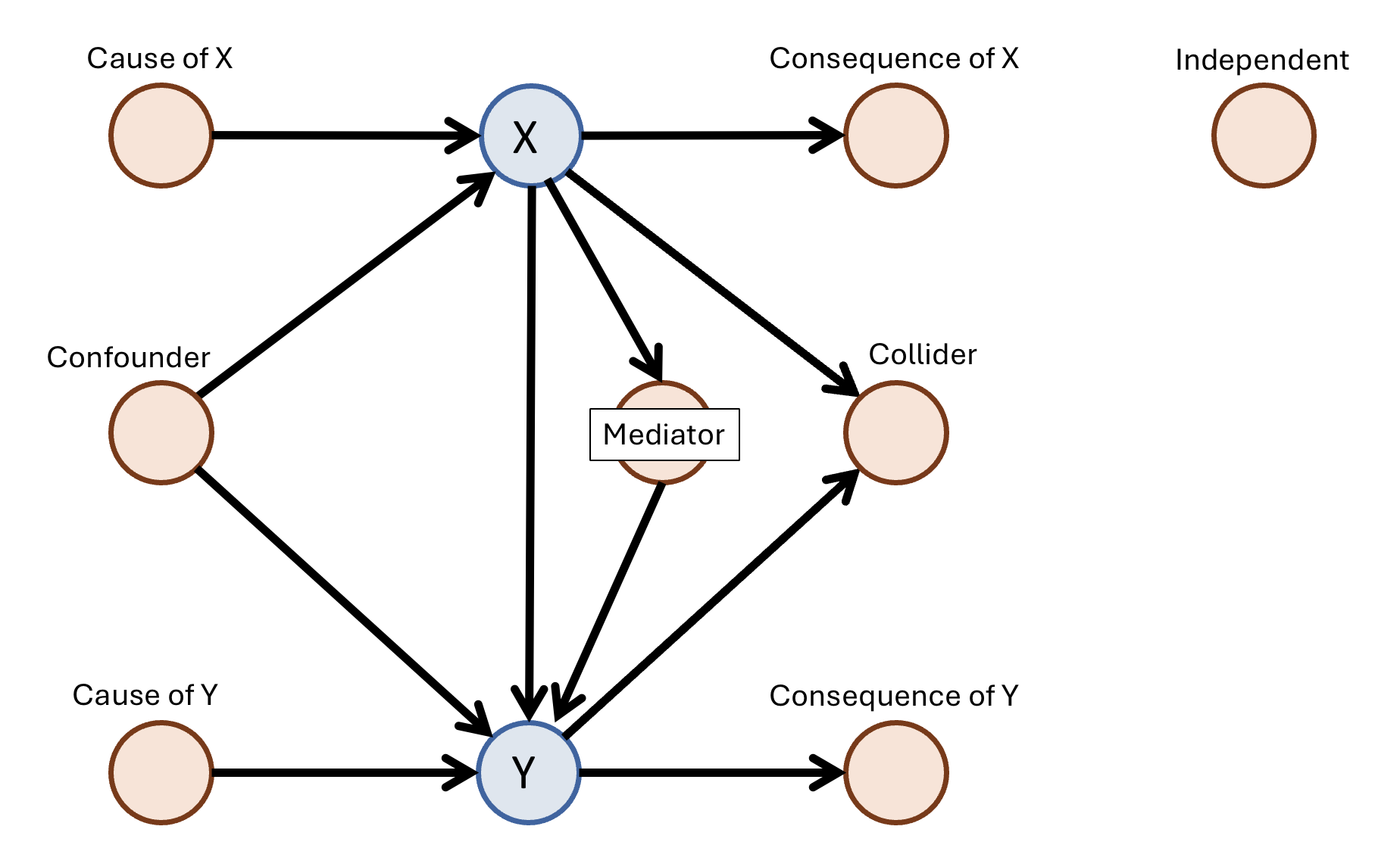 The 8 causal role classes (image from the ADIA Lab paper)
Metric: balanced accuracy — mean per-class recall. Overall accuracy is never reported. The hardest classes are Collider and Mediator; they count equally with the easy ones.
Baseline: The Top-1 Solution
Input Representation
The top-1 solution’s core insight is representing each variable pair as a sorted observation curve rather than a set of scalar statistics.
For each directed pair $(u, v)$ where $u \neq v$, sort all 1000 observations by $u$’s values to get a permutation index sort_idx. Reading every other variable at that permutation gives a length-1000 functional curve of how $v$ behaves as $u$ increases — the conditional curve $v \mid u$. Any scalar summary permanently discards the shape of this curve. Conv1D reads it directly.
The baseline builds 3 channels per directed edge $(u, v)$, all at the sorted permutation:
| Channel | What it is |
|---|---|
| $\mathbf{c}_1$ | $u$ sorted by $u$ — the sorted values of the source variable |
| $\mathbf{c}_2$ | $v$ sorted by $u$ — the conditional curve of $v$ given $u$ |
| $\mathbf{c}_3$ | Multivariate kernel regression coefficient $\hat{\beta}^{(h=0.5)}_{u \to v}$ at the sorted permutation — predicts $v$ from all other variables simultaneously |
For a graph with $p$ variables this produces $E = p(p-1)$ directed edges, each a tensor of shape $(3, 1000)$.
Each edge also has a type label (7 types, encoding that edge’s structural relationship to the anchor $X \to Y$, e.g. $X \to v$, $v \to Y$, other $\to$ other, etc.).
Pipeline
Step 1 — Conv1D encoder: Each $(3, 1000)$ edge tensor goes through a Stem layer (linear projection from 3 to $d$ channels) followed by 5 residual Conv1D blocks, then AdaptiveAvgPool1d. Output: one $d$-dim embedding per edge.
Step 2 — Edge type fusion: The 7 edge types are projected to $d$-dim vectors via a learned embedding table. These are merged with the Conv1D output via a linear fusion layer. Output: one $d$-dim embedding per edge encoding both content and structural type.
Step 3 — Self-attention: Two self-attention layers run over all $E$ edge embeddings simultaneously. Each edge can attend to all other edges, enabling global graph reasoning. Output: $E$ attended edge embeddings.
Step 4 — Two heads:
- Edge head (
Linear(d, 2)): predicts whether a directed causal edge $u \to v$ actually exists in the ground truth DAG — binary classification, trained with cross-entropy against the adjacency matrix. This is an auxiliary loss, discarded at inference. - Node head (
Linear(d, 8)): for each non-$X$/$Y$ node $v$, gathers the 4 attended edge embeddings at positions $(v \to X), (v \to Y), (X \to v), (Y \to v)$, merges them via a linear fusion, and produces the 8-class causal role prediction.
The combined training loss is:
\[\mathcal{L} = \mathcal{L}_{\text{node}} + \lambda \cdot \mathcal{L}_{\text{edge, binary}}\]The edge head’s binary objective (edge exists or not) is well-defined and has clean ground truth from the adjacency matrix. It forces the Conv1D + attention stack to produce embeddings that are sensitive to actual causal structure, ensuring the node head receives informative input rather than unconstrained representations.
My reimplementation: 73.96% local / 73.6% leaderboard (vs. claimed 76.70%). The gap is likely due to implementation details not fully specified in the writeup.
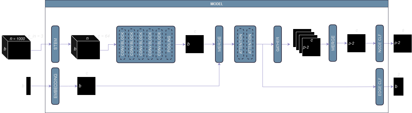 The baseline architecture (image from the top-1 writeup)
Contribution 1: Multi-Bandwidth Kernel Channels
The baseline uses a single bandwidth $h=0.5$ for the kernel regression coefficient. A single bandwidth creates a bias-variance tradeoff — coarse $h$ smooths away local nonlinear structure, fine $h$ is noisy.
I add coefficients at two additional bandwidths, giving the model simultaneous access to local and global conditional structure. The total channel count grows from 3 to 5:
\[[\text{sort}_u(u),\ \text{sort}_u(v),\ \hat{\beta}^{(h=0.2)},\ \hat{\beta}^{(h=0.5)},\ \hat{\beta}^{(h=1.0)}]\]All channels are at the same sorted permutation, so they are spatially aligned sequences that Conv1D can jointly process.
Result: 73.96% → 75.44% (+1.48%)
Contribution 2: ANM Residual Channels
The Additive Noise Model [Hoyer et al., 2009] gives a testable prediction: if $u$ truly causes $v$, then the residuals of regressing $v$ on $u$ and other variables should be statistically independent of $u$. The reverse direction residual will not be independent — it will retain structure. This asymmetry is a direct signal of causal direction.
I compute multivariate kernel regression residuals for each directed edge $(u, v)$ at 3 bandwidths and add them as 3 additional channels at the sorted permutation:
\[[\epsilon_{u \to v}^{(\sigma=1.0)},\ \epsilon_{u \to v}^{(\sigma=2.0)},\ \epsilon_{u \to v}^{(\sigma=4.0)}]\]This brings the total to 8 channels: 2 raw sorted values + 3 kernel coefficients + 3 ANM residuals, all length-1000, all sorted by $u$.
Why this helps specific classes: A Collider ($X \to K \leftarrow Y$) and a Consequence of X ($X \to K$) both have $X$ causing $K$. For the correct direction, regressing $K$ on $X$ leaves residuals that are near-independent of $X$ — a flat residual curve when sorted by $X$. The reverse direction residual retains structure. The model learns to read this asymmetry across the 8 residual channels. Empirically, Collider and Consequence of X recall improved most.
Result: 75.44% → 76.94% (+1.50%). Combined with XY augmentation: 80.26% / 80.22% LB.
 The 8-channel edge representation
Contribution 3: XY Augmentation
Idea from top-3 writeup.
In the original setup, the model always sees each graph with fixed $(X, Y)$ labels. This risks learning positional shortcuts — “when I see this pattern, $X$ is usually at index 0” — rather than the underlying topology.
XY augmentation relabels graphs so the same underlying structure is presented from multiple anchor perspectives. Any pair of variables with a directed causal edge between them can be relabeled as the new $(X’, Y’)$ anchor, and all other variables’ roles are recomputed accordingly. A graph with $p$ variables yields roughly 11 valid relabelings on average. This forces the model to learn the topological role of each variable relative to the anchor edge, not relative to fixed label positions.
The effective training set grows from 25K graphs to 263K augmented samples.
Interaction with structural bias: XY augmentation gave +3.32% on v8b but only +1.55% on v11. Both techniques encode the same information — that $X$ and $Y$ are topological anchors, not positional constants — but one does it through data diversity and the other through architecture. Once the structural bias is in place, augmentation has less new information to contribute. The partial redundancy is indirect evidence that the structural bias mechanism is functioning correctly.
 Demonstration of the augmentation process (image from top-3 writeup)
Contribution 4: Structural Attention Bias
This is the only architectural change that produced a significant positive result.
Standard self-attention treats every pair of edge embeddings $(e_i, e_j)$ identically in computing attention scores. But in a causal graph, the topological relationship between two directed edges carries strong prior information. Two edges forming a chain $X \to K \to Y$ should interact differently from two completely unrelated edges.
I define 6 topological relationship types between any pair of directed edges $(u_1 \to v_1)$ and $(u_2 \to v_2)$:
| Type | Condition |
|---|---|
| Reverse | $u_1 = v_2$ and $v_1 = u_2$ |
| Shared source (fork) | $u_1 = u_2$, not reverse |
| Shared target (collider) | $v_1 = v_2$, not reverse |
| Forward chain | $v_1 = u_2$, not reverse |
| Backward chain | $u_1 = v_2$, not reverse |
| Unrelated | none of the above |
A learned scalar bias $b_{\tau, h} \in \mathbb{R}$ per type $\tau$ per attention head $h$ is added to the attention logit before softmax:
\[A_{ij}^{(h)} = \frac{\mathbf{q}_i^{(h)} \cdot \mathbf{k}_j^{(h)} + b_{\tau(i,j), h}}{\sqrt{d_h}}\]The biases are zero-initialized, so the model starts from standard attention and learns to prioritize topological relationships during training. Total additional parameters: 24 scalars (6 types × 4 heads).
Why this works where other architectural changes failed: Every other architectural addition I tried (cross-attention branches, dual-path transformers, node-centric pooling) degraded performance. Those changes added raw capacity without a problem-specific prior, leading to overfitting on 25K samples. The structural bias adds almost no capacity — it only learns how much to weight each topological relationship type, with the types themselves defined by causal graph theory. The inductive bias is entirely appropriate to the problem.
Result: v8b 76.94% → v11 79.59% (+2.65%). With XY augmentation: 81.14% local / 80.82% LB.
 The structural attention bias: a learned scalar per (type, head) pair is added to the attention logit
What Didn’t Work
ML fullstack (v13): 72.64%
I built a complete machine learning pipeline — 300+ engineered features (pairwise correlations, partial correlations, mutual information, outputs from PC, LiNGAM, NOTEARS, ANM), three gradient boosting models, a GNN refinement stage, and a stacking ensemble. Result: 72.64% — below the simple Conv1D baseline at 73.96%.
Why: Scalar feature compression is irreversible. Once you summarize a 1000-point conditional expectation curve into a single number, you permanently discard its shape — curvature, heteroscedasticity, nonlinearity. That shape is exactly what distinguishes a Mediator from a Consequence of X. Conv1D reads the full curve; no amount of scalar engineering can recover what was thrown away. I also tried injecting these scalars as a parallel tower into the deep learning model — this also failed, because broadcasting a scalar across a length-1000 sequence gives it no structural relationship to the sequence positions.
Architectural complexity (v3, v4, v6): regressed 1–2%
Cross-attention branches and dual-path transformers all degraded performance. Architectural complexity only helps when it encodes an appropriate inductive bias. General capacity additions overfit on 25K training samples.
Node-centric attention (v9, v9b): lost ~1.5%
Compressing the $O(p^2)$ edge context to node-level summaries consistently underperformed. Full edge self-attention is load-bearing: global graph reasoning requires seeing all pairwise relationships simultaneously.
Score Progression
| Version | Local BA | LB | Key change |
|---|---|---|---|
| Baseline reimplementation | 73.96% | 73.6% | — |
| + multi-bandwidth kernel (v5m) | 75.44% | 74.98% | +1.48% |
| + ANM residuals (v8b) | 76.94% | — | +1.50% |
| + XY augmentation (v8b+) | 80.26% | 80.22% | +3.32% |
| + structural bias, no aug (v11) | 79.59% | — | +2.65% over v8b |
| + XY augmentation (v11+) | 81.14% | 80.82% | best result |
Summary
Four contributions, each with a clear mechanistic motivation:
- Multi-bandwidth kernel channels — simultaneous access to local and global conditional structure
- ANM residual channels — direct causal direction signal, most impactful for Collider and Consequence classes
- XY augmentation — forces topology learning over position learning, +3.32% on v8b
- Structural attention bias — encodes causal graph priors into attention with 24 parameters, +2.65% over v8b
The core lesson: representational form matters more than model complexity. Full functional curves contain information that no scalar feature set can recover. Architectural changes only help when they carry an appropriate inductive bias — general capacity additions hurt.
References
- thetourney. ADIA Lab Causal Discovery Challenge — 1st Place Solution. 2024. link
- mutian-hong. ADIA Lab Causal Discovery Challenge — 3rd Place Solution. 2024. link
- Hoyer, P. et al. Nonlinear Causal Discovery with Additive Noise Models. NeurIPS 2009.
- Pearl, J. Causality: Models, Reasoning, and Inference. Cambridge University Press, 2009.
- Olivetti, E. et al. Can Machines Learn Causal Structure? Evidence from ADIA Lab’s Causal Discovery Challenge. SSRN 2025.